User Documentation Molecular Usecase

This is the user documentation for the QuCUN material science use case. In the material science use case the quantum computer is used to obtain the ground state energy and derived properties of a molecule consisting of two atoms. It is an example of simulation use cases for quantum computers where the quantum computers can be used to solve an inherently quantum simulation problem that in general would require exponential resources on a convetional computer. This user documentation gives a general introduction of the use case and the methods used here.

Table of Contents

• Introduction
• Molecular Dissociation
• Variational Quantum Eigensolver (VQE)
• Implementation Details

Introduction

An important property of molecules is the dissociation profile, the ground state energy of the molecule over the distance between two atoms in the molecule. From the dissociation profile, properties like the dissociation energy, the equilibrium distance in the molecule and the oscillation frequency of the atoms in the molecule can be obtained.

In this use case, we limit ourselves to the simple case of a molecule consisting of two atoms. For this case, the definition of the distance is clear and the number of molecular orbitals that needs to be involved in the calculation can be small enough to fit on a quantum computer.

The dissociation profile is obtained from the quantum computer using a VQE (Variational Quantum Eigensolver) with a Unitary Coupled-Cluster Single Double (UCCSD) ansatz. VQE is a variational approach, which means that this is a hybrid algorithm where free parameters of the VQE algorithm are optimized by a classical optimizer during run time. For a more detailed discussion of the quantum algorithm used in this use case, see the VQE section.

The quantum solver is based on the qiskit library, which provides a general quantum computing toolkit as well as a selection of quantum algorithms (like the VQE) and ansätze for the VQE.

The derived properties (equilibrium distance r0, dissociation energy ΔE and oscillation frequency ω) are obtained by pure classical post-processing fitting the VQE dissociation profile to the Morse Potential. For an example for extracting the properties for a Hydrogen atom, see the Dissociation profile section.

As a variational method, the quality of the results of the VQE can strongly depend on the exact parameters chosen for the calculation.

Molecular Dissociation

Dissociation profile for the hydrogen molecule

In this materials use case the VQE algorithm is used to calculate the ground state energies of a molecule across different interatomic distances on a quantum computer. The so obtained dissociation profile of the molecule (here: H2) is compared to the results obtained from the pure Hartree Fock method and to the conventional full CI calculation (referred to as "exact" here).

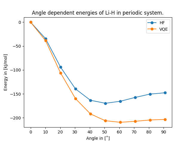
This plot shows a dissociation profile for the hydrogen molecule calculated in the 6-31g (reduced) basis, where orbitals [2, 3] have been removed from the active space making it a minimal basis set to reduce calculation runtime. Similar to the conventional methods of quantum chemistry, a small basis set leads to a limited precision of the obtained results.

As one can see from a simple demonstration, the obtained results from the quantum algorithm (here: VQE) show a good agreement with the (exact) full CI calculation. Moreover, its accuracy (here: on an ideal quantum computer) is much higher than of the classical Hartree Fock method, which has been used as the initial ansatz here. Also the true equilibrium distance (vertical dotted line) and the expected dissociation limit (horizontal dotted line) can be described with a sufficient quality, although only a minimal basis set was used for the calculations.

Molecule properties

The obtained VQE dissociation curve allows us to derive important molecule properties, like equilibrium distance r0, dissociation energy ΔE and oscillation frequency ω by pure classical post-processing. The use case extracts these properties by fitting the Morse Potential to the dissociation curve obtained from the VQE (or to the other results obtained from the use case).

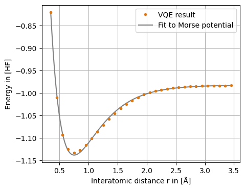
We see that the VQE (Hartree-Fock, exact) results can be fitted quite nicely by the Morse Potential.

The desired molecule properties, like equilibrium distance r0, dissociation energy ΔE and oscillation frequency ω, can be obtained analytically from the Morse Potential fit.

Specifically for the given example, given the limited precision when running measurements with minimal basis sets, the quantum algorithm (on a perfect simulated quantum computer) achieves results of a similar quality as the classical full CI calculation.

Dissociation energy from thermodynamic cycle

There exists an alternative way to compute the dissociation energy of the hydrogen molecule as the heat effect of the reaction: \( H_2 \longrightarrow 2H \). The dissociation energy is then computed as follows: \( \Delta E = 2E(H) - E(H_2) \), where \( E(H) \) is the energy of a single hydrogen atom, while \( E(H_2) \) is the energy of the hydrogen molecule at the minimum of the potential energy curve. Since the hydrogen atom has only one electron, there is no electron correlation, and \( E(H) \) should be calculated with the Hartree-Fock method for all three approaches (VQE, Hartree-Fock, and exact). However, the molecule should be computed with the electronic structure method of choice. It is instructive to compare \( \Delta E \) obtained by this method with the one obtained from the fitted Morse potential.

The reference values for the properties of interest for the Hydrogen molecule from the literature are (see also ref 1):

Notes

Please note that for demonstrative purposes a small molecule has been chosen here, which allows to compare the VQE results to the exact solution.
The VQE calculations shown here ran on a quantum computing simulator, not on real quantum computer hardware yet. This implies the assumption of an ideal, i.e. error-free, quantum computer. Whereas real quantum computers are subject to so called 'noise' (errors) that affects the obtained results. Results from runs on actual hardware will deviate more strongly from the exact solution.

Variational Quantum Eigensolver (VQE)

The Variational Quantum Eigensolver (VQE) is hybrid quantum-classical algorithm that can be used to calculate ground state energy of a Hamiltonian (e.g. a molecule) on a quantum computer.

The core principle of the VQE is the variational principle. The ground state is the lowest energy state \(|\psi_0 \rangle \) of all possible states \( \{ |\psi \rangle \}\) of a Fock space, where the energy is the expectation value of a Hamiltonian \(H \). Finding the lowest energy state of a given set of trial states \( \{ |\psi_T \rangle \}\) is a good approximation to finding the ground state and the ground state energy as long as the set of trial states covers the Fock space densely enough that a trial state is close to the true ground state.

The VQE uses the quantum computer to prepare the trial states \( |\psi_T(\theta) \rangle \) as a function of some classical parameters \(\theta \). The expectation value of the Hamiltonian is then measured on the quantum computer as well. The hybrid part of the VQE is a classical optimizer. The classical optimizer tries to minimize the cost function, the expectation value of the Hamiltonian, by varying the classical parameters \(\theta \). Once converged to an optimal set of parameters \(\theta_0\) the approximation of the ground state is given by \[ | \psi_0 \rangle \approx | \psi_T(\theta_0) \rangle \] and the approximation of the ground state energy is given by the final value of the cost function. Besides the ansatz for the trial wave functions, the chosen optimizer can have a large influence on the quality of the VQE results. For a list of the available optimizers see section Implementation Details.

For a detailed discussion of the Variational Quantum Eigensolver, we refer the reader to paper by McClean et al..

Ansatz

As mentioned above, the ansatz for the trial wave functions is an important choice for the VQE algorithm. We use the Unitary Coupled-Cluster Singles and Doubles (UCCSD) ansatz for the VQE algorithm. This ansatz is a standard choice for the VQE algorithm when considering quantum chemistry problems and is implemented in qiskit. The ansatz state is constructed starting from a Hartree-Fock state, and then acting on it with some exponential "cluster" operators that generate excitations to account for electron correlation. Electron correlation built this way accounts for electron-electron repulsion better than the average field used by Hartree-Fock. More precisely, while Hartree-Fock only includes exchange correlation between electrons (i.e. the correlation due to antisymmetry, also known as Fermi correlation), the UCCSD ansatz improves on it by partially accounting for Coulomb correlation.

The wavefunction of the coupled-cluster theory is written as an exponential ansatz: \[ | \psi \rangle = e^T | \Phi_0 \rangle \] where \( | \Phi_0 \rangle \) is a Slater determinant obtained from Hartree-Fock molecular orbitals. The action of the exponentiated cluster operator \( T \) on the state \( |\Phi_0\rangle \) produces a linear combination of Slater determinants that partly account for Coulomb interaction.

The cluster operator has the form \( T = T_1 + T_2 \) , where \( T_1 \) generates single-electron excitations and \( T_2 \) generates two-electron excitations, from which the naming "Singles and Doubles" in the UCCSD acronym stems. The expressions for the excitation operators are \[ T_1 = \sum_{ia} t_{ia} c^{\dagger}_a c_i + h.c. \] \[ T_2 = \frac{1}{4} \sum_{ijab} t_{ijab} c^{\dagger}_a c^{\dagger}_b c_i c_j + h.c. \] where \( t_{ia} \) and \( t_{ijab} \) are real coefficients, \( c^{\dagger} \) and \( c \) are fermionic creation and annihilation operators, and the indices \( i, j \) correspond to occupied molecular orbitals in the original Hartree-Fock state \( | \Phi_0\rangle \), while \( a, b \) correspond to unoccupied states. The \( t_{ia} \) and \( t_{ijab} \) are the free parameters that are optimized by the classical optimizer to find the minimum energy.

While the operators \( T_1 \) and \( T_2 \) generate respectively single and double excitations when acting directly on \( |\Phi_0\rangle \), notice that when exponentiated as \( e^T \) it also generates higher correlations due to the power series expansion of the exponential.

Implementation

In this section we discuss the implementation details of the use cases and the available options that can be chosen by the (expert) user.

The use cases is implemented in Python with the qiskit quantum computing framework. The use case will run on the QuCUN platform. Whether it runs on a noise-less quantum simulator, a noisy quantum simulator or on actual quantum hardware is determined by the QuCUN platform settings. When running on an ideal, i.e. error-free quantum computer simulator, the simulation results can be very accurate, depending on the chosen parameters. Real quantum computer hardware is subject to environmental noise (leading to errors) that affects the obtained results negatively.

Chemical drivers and basis choices

The UCCSD ansatz used by the use case needs the Hartree-Fock self consistent solution of the molecule as an input. This solution can be obtained by qiskit from a chemical driver. The use case supports two chemical drivers: PySCF and Psi4. The default choice for a chemical driver to perform the Hartee-Fock calculation is PySCF.

The chemical driver takes the input molecule, as well as the information on the basis set, to define the electronic structure problem.

In computational chemistry, a basis set is a finite set of functions, usually chosen to be orthogonal, that are used as a basis to approximate electronic wavefunctions. As the number of basis functions in the set approaches infinity, the accuracy of the approximation of the electronic wavefunction calculated using the basis set improves at the price of a higher computational cost.

Basis sets are used for example to calculate the molecular orbitals that serve as the Hartree-Fock starting point for the construction of the UCCSD ansatz, but also to construct the ansatz from the initial Hartree-Fock state. The choice of basis set is influenced by the tradeoff between computational resources available and accuracy of the desired result. A basis set is called minimal if for each atom in the molecule it contains only enough orbitals to contain the electrons in the neutral atom. Thus for the hydrogen atom only a single 1s orbital is needed, while for a carbon atom, 1s, 2s and three 2p orbitals are needed. The basis sets available are:

• STO3G: Minimal basis set in which each basis function is expressed as a linear combination of 3 primitive Gaussian functions. Both core and valence orbitals are represented in this way. Allows for fastest but least accurate calculations. To keep runtimes of simple test runs low, this is the default option.
• 6-31G: Split-valence basis set, i.e. the core orbitals and the valence orbitals are represented differently. Here, the core orbitals are represented as a linear combination of six Gaussian functions, while the valence orbitals are represented with two basis functions, expressed as linear combinations of respectively three and one primitive Gaussian function. Gives more accurate results but has longer run times.
• MINAO (MINimal Atomic Orbital) : Tradeoff between accuracy and computational cost.

Classical Optimizers

The cost function that we want to minimize is the expectation value of the fermionic Hamiltonian of interest, evaluated in the UCCSD ansatz state with a certain set of parameter values. The parameter values are then optimized by a classical optimizer. The classical optimizers available are:

• L-BFGS-B (Limited-memory BFGS Bound): It is a limited-memory approach, meaning that doesn't explicitly store the Hessian matrix, which can be computationally expensive for large-scale problems. Instead, it maintains an approximation of the inverse Hessian matrix using limited memory. This makes it suitable for optimization problems with a large number of variables. As a gradient-based optimizer L-BFGS-B gives good results for noise-less quantum simulator but is sensitive to noise in the cost function due to noise on the quantum computer.
• COBYLA (Constrained Optimization BY Linear Approximations): COBYLA belongs to the class of direct search or derivative-free optimization methods. This means that it does not rely on gradient information (first or second derivatives) of the objective function or constraints. Instead, it uses a pattern of linear approximations to estimate the direction of descent or ascent in the objective function space while respecting the constraints. As such, COBYLA is particularly useful when the objective function or constraint functions are noisy, non-smooth, or difficult to compute derivatives for. For this reason, we use COBYLA as the default optimizer as it is suitable for actual quantum computing hardware, where we encounter noise in the quantum computer.
• SLSQP (Sequential Least Squares Quadratic Programming): SLSQP utilizes gradient information (first derivatives) of the objective function and constraints, if available. This makes it an efficient choice for optimization problems with smooth functions where gradient information can be computed or approximated. SLSQP employs a sequential quadratic programming approach, which involves approximating the objective function and constraints with quadratic models and then iteratively solving subproblems to optimize these models within the constraint boundaries. This process continues until convergence to the optimal solution.
• SPSA (Simultaneous Perturbation Stochastic Approximation): SPSA is a derivative-free optimization method that falls under the umbrella of stochastic approximation techniques. SPSA does not require gradient information (first or second derivatives) of the objective function. Instead, it approximates the gradient by perturbing the decision variables simultaneously and using finite differences to estimate the change in the objective function.
• NFT (Nakanishi-Fujii-Todo): It is a sequential minimal optimization method specifically designed for hybrid quantum-classical algorithms.
• CG (Conjugate Gradient): An iterative numerical optimization algorithm used for solving unconstrained optimization problems, particularly those that involve quadratic objective functions. CG is an iterative method, which means it refines an initial guess for the solution in a series of steps. It does not require the explicit calculation or storage of the Hessian matrix, making it suitable for large-scale problems.

In the official SciPy documentation additional information on some of these optimizers is available.

Qubit Mapper

The qubit mapper translates the fermionic degrees of freedom in the original quantum chemisty problem into spin degrees of freedom that can be represented on a quantum computer. Several different mappings are possible, in qiskit we have two options

• ParityMapper - Encodes the parity of all teh fermionic orbitals up to an orbital j in qubit j. When providing the overall number of fermionic particles in the system, the qiskit ParityMapper can reduce the number of qubits by 1. We use this mapping as the default.
• JordanWigner - The JordanWigner mapping encodes the occupation of an fermionic orbital j in qubit j.

For a more detailed discussion of mappings in the context of quantum simulation see for example this paper by Seeley et al.

Inactive orbitals

The number of required qubits in the system increases linearly with the number of molecular orbitals in the problem. When the number of qubits becomes too large for the available hardware the number of qubits required can be reduced by reducing the active space. Orbitals that are always occupied and orbitals that are always unoccupied are removed from the problem in a transformation. Removing orbitals from the active space speeds up calculations, but depending on the molecule being simulated can impact the accuracy of the results. Core orbitals are always removed from the active space automatically. The user can additionally remove unoccupied orbitals with the inactive_orbitals orbitals option that lists the orbitals that should be removed as unoccupied by the transformation. Qiskit does not perform a check when removing the unoccupied orbitals and this option should only be used by expert users. For details on the mathematical transformation involved see.

Calculated results

For better comparison the use case calculates three results for the dissociation profile and the post-processing:

• The VQE result
• The Hartee-Fock result taken directly from the chemical driver
• The exact> solution. The exact solution corresponds to solving for the ground state of the effective Hamiltonian obtained from the chemical driver by exact diagonalisation. In chemical terms it would be equivalent to Full CI, but it is not a direct diagonalisation of the original fermionic Hamiltonian.

Ressources

[1] Experimental data for H2 , https://cccbdb.nist.gov/exp2x.asp?casno=1333740
[2] Scientific paper on the improved theoretical ground state energy of the hydrogen molecule
[3] Scientific paper on the potential energy curves

Materials Use Cases: Optimal orientation in periodic materials

This user documentation delves into the QuCUN material science use case focused on investigating the optimal orientation of atoms within a periodic material system. Specifically, it explores a model case involving a one-dimensional lattice essentially a wire composed of two distinct types of atoms in its unit cell, exemplified by Li and H. This scenario showcases how quantum computing can be pivotal in addressing complex simulation challenges, particularly in material science where understanding atomic arrangements in periodic structures is crucial. Through this use case, we demonstrate the potential of quantum computers to accurately determine ground state energies and related properties of molecular systems. Such tasks, owing to their quantum nature, often demand resources beyond the practical reach of classical computing architectures. Herein, we provide an overview of the approach and methodologies employed in this quantum simulation use case, highlighting the innovative use of quantum computing to surmount barriers faced by traditional computational methods.

Table of Contents

• Background
• Implementation

Background

Here we want to give a simple toy model for a material science use case in a periodic system. We are considering a one-dimensional lattice (a wire) with two atoms of distinct elements in the unit cell (for example Li and H). The lattice can be described by atomic coordinates and basis vectors. The atomic coordinates define the position of a Li and a H atom with respect to each other and basis vectors define the unit cell containing the atoms and repeated periodically along the x-axis.

We are interested in finding the optimal orientation of the atoms in the unit cell. Specifically, we want to find the optimal angle of the axis connecting the atoms in the unit cell to the lattice vector of the periodic direction. Without loss of generality, we assume that the system is periodic along the x-axis, the first atom of element A is located at (0,0,0) in the unit cell, and the second atom of element B has a constant distance to the A atom and is rotated in the x-y plane. We are looking for the optimal angle with respect to the x-axis.

This application is a model case to study polymorphism and phase transitions in crystals. Restricted to one-dimensional parameter space (rotation angle) we are looking for stable orientations of the atoms in the cell. These are located at the energy minima and correspond to the phases (polymorphs), whereas energy maxima define the phase transition barriers.

As in other use case we set up the system the problem that is solved in two steps. First some classical pre-processing is performed using a computational chemistry software package (PySCF in this case). Then the output of the pre-processing is handed to a variational quantum eigensolver (VQE) that can run on a real quantum computer or on a simulated quantum computer. The VQE on the quantum computer is again used to find the ground state of a finite size Hamiltonian. The periodicity only enters the problem when preparing the Hamiltonian used in the VQE with the classical preprocessing.

PySCF allows us to define a periodic system by defining the unit cell and the basis vectors. In the periodic system, the atoms in the unit cell are able to interact with the atoms of the other unit cells. The classic pre-processing part of the use case uses a Hartree-Fock method to determine the approximate solution of the molecular orbitals taking into account the interaction between unit cells but without taking into account electron-electron correlation.

The Hartree-Fock method produces a Hamiltonian of the atoms in one unit cell that already accounts for the interaction between unit cells and also produces approximate ground state energies. The Hamiltonian produced by the periodic Hartree-Fock calculation can then be passed to the VQE without modifying the VQE for periodicity.

Implementation details

The implementation details are similar to the molecular use case. The code has been implemented based on the qiskit quantum computing framework and with the help of PySCF.

In setting up the problem the same optimizers are available as for the molecular use case . The available qubit encodings that encode the electronic degrees of freedom into qubits are also the same (Parity encoding and Jordan-Wigner encoding).

Basis choices

In the periodic problem we have more choices, because PySCF has some specific orbitals for periodic systems.

• GTH_SZV A basis set consisting of Gaussian functions optimized for periodic systems and to be used with pseudopotentials. SZV: single-zeta valence, i.e. one contracted function per orbital. To keep runtimes of simple test runs low, this is the default option.
• GTH_DZVP A basis set consisting of Gaussian functions optimized for periodic systems and to be used with pseudopotentials. DZV: double-zeta valence, i.e. two contracted function per orbital plus a set of polarization functions.
• STO3G: Minimal basis set in which each Slater-type basis function is expressed as a linear combination of 3 primitive Gaussian functions. Both core and valence orbitals are represented in this way. Allows for fastest but least accurate calculations. For Li-H this gives better results that default option but takes considerably longer
• 6-31G: Split-valence basis set, i.e. the core orbitals and the valence orbitals are represented differently. Here, the core orbitals are represented as a linear combination of six Gaussian functions, while the valence orbitals are represented with two basis functions, expressed as linear combinations of respectively three and one primitive Gaussian function. Gives more accurate results but has longer run times.
• MINAO (MINimal Atomic Orbital) : Tradeoff between accuracy and computational cost.

PySCF also allows the use of pseudopotentials. In the use case two configurations are allowed

• Off No pseudopotential is used in the quantum chemistry calculation.
• GTH_PADE Goedecker-Teter-Hutter dual-space pseudopotential to be used with GTH-basis sets.

Calculated results

As for the molecular calculation, Hartree-Fock energies, VQE energies and exact diagonalisation energies are calculated for the angle-dependent ground states electronic energies. Since we are interested in the optimal orientation of the two atoms in the unit cell, we determine the angles that correspond to the energy minima and the height of the energy barrier between them in post processing.

In the following you can see the angle dependent ground state energies for Li-H in a 1D periodic system with a Li-H distance of 1.6 Å and with a periodic cell of length 3.2 Å.

Here, we observe a stable phase at 50 (HF) and 60 (VQE) °:

We observe two transition state structure:

1. At 0 ° (higher barrier)

2. At 90 ° (lower barrier)

Account of electron correlation with VQE shifts the stable structure by 10 ° as compared to HF. This potential curve is mirror-symmetric when continued towards 180 °, giving and equivalent minimum at 140 (HF) or 150 (VQE) °. In addition, the depth of the potential well is larger at the VQE level (209 kJ/mol) than at the HF level (170 kJ/mol). At the same time, the barrier at 90 ° between equivalent tilted stable structures is lower for VQE (6 kJ/mol) than for HF (22 kJ/mol). This can be interpreted as follows: electron correlation (VQE) makes structures more stable, but more flexible, so that the system constantly switches between equivalent minima.